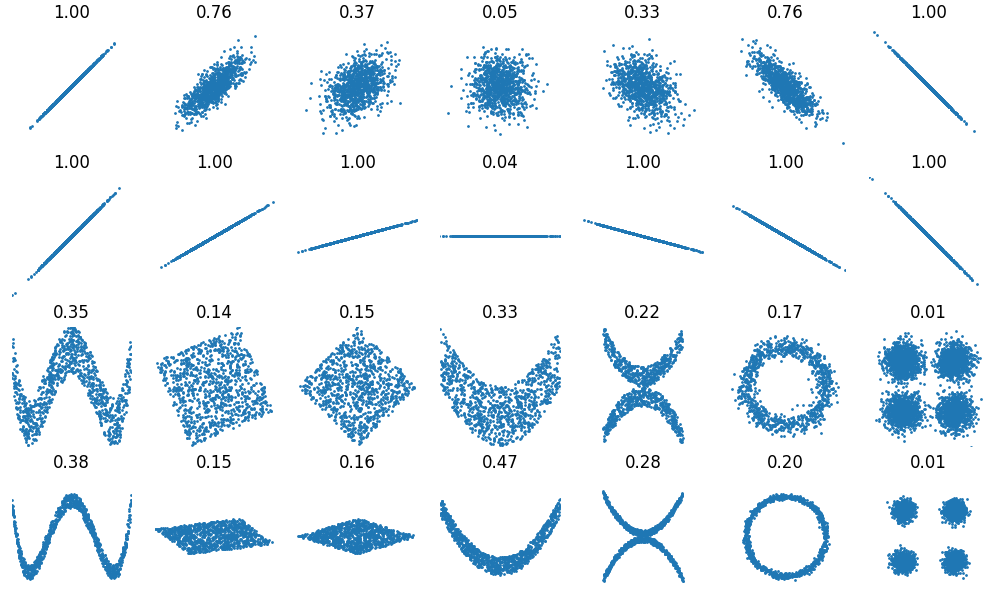
Distance correlation plot

Plot 2d synthetic datasets and compute distance correlation between their coordinates.

The objective of this example is to replicate the results obtained in the Wikipedia page for distance correlation.

We first include the necessary imports.

import matplotlib.pyplot as plt
import numpy as np
import scipy.stats

import dcor

We now create a random generator with a fixed seed for reproducibility. We also define the number of samples per dataset. Both will be global variables for this script.

random_state = np.random.default_rng(seed=123456789)
n_samples = 1000

We now define utility functions for plotting the data and generating the synthetic datasets.

def plot_data(x, y, ax, xlim, ylim):
    """Plot the data without axis."""
    ax.set_title(f"{correlation:.2f}")
    ax.set_xlim(xlim)
    ax.set_ylim(ylim)
    ax.scatter(x, y, s=1)
    ax.axis(False)

The first row of datasets is composed of bivariate Gaussian distributions with different correlations between the coordinates, so we define a function that returns one of these datasets given the desired correlation.

def gaussian2d(correlation):
    """Generate 2D Gaussian data with a particular correlation."""
    return random_state.multivariate_normal(
        mean=[0, 0],
        cov=[[1, correlation], [correlation, 1]],
        size=n_samples,
    )

The second row of datasets have the data in a line with different rotations. We now define a function for rotating a dataset by a given number of degrees. That rotation is performed using a rotation matrix.

def rotate(data, angle):
    """Apply a rotation in degrees."""
    angle = np.deg2rad(angle)
    rotation_matrix = [
        [np.cos(angle), - np.sin(angle)],
        [np.sin(angle), np.cos(angle)],
    ]

    return data @ rotation_matrix

The two final rows of datasets consist of data with complex relationships between the coordinates. The difference between these rows is the spread of the data, so we make that a parameter. We have made this function a generator that yields each dataset one at a time, in order to simplify looping over the datasets. As each distribution has different support, we make sure to yield not only the data, but also the limits for plotting.

def other_datasets(spread):
    """Generate other complex datasets."""
    x = random_state.uniform(-1, 1, size=n_samples)
    y = (
        4 * (x**2 - 1 / 2)**2
        + random_state.uniform(-1, 1, size=n_samples) / 3 * spread
    )
    yield x, y, (-1, 1), (-1 / 3, 1 + 1 / 3)

    y = random_state.uniform(-1, 1, size=n_samples)
    xy = rotate(np.column_stack([x, y]), -22.5)
    lim = np.sqrt(2 + np.sqrt(2)) / np.sqrt(2)
    yield xy[:, 0], xy[:, 1] * spread, (-lim, lim), (-lim, lim)

    xy = rotate(xy, -22.5)
    lim = np.sqrt(2)
    yield xy[:, 0], xy[:, 1] * spread, (-lim, lim), (-lim, lim)

    y = 2 * x**2 + random_state.uniform(-1, 1, size=n_samples) * spread
    yield x, y, (-1, 1), (-1, 3)

    y = (
        (x**2 + random_state.uniform(0, 1 / 2, size=n_samples) * spread)
        * random_state.choice([-1, 1], size=n_samples)
    )
    yield x, y, (-1.5, 1.5), (-1.5, 1.5)

    y = (
        np.cos(x * np.pi)
        + random_state.normal(0, 1 / 8, size=n_samples) * spread
    )
    x = (
        np.sin(x * np.pi)
        + random_state.normal(0, 1 / 8, size=n_samples) * spread
    )
    yield x, y, (-1.5, 1.5), (-1.5, 1.5)

    xy = np.concatenate([
        random_state.multivariate_normal(
            mean,
            np.eye(2) * spread,
            size=n_samples,
        )
        for mean in ([3, 3], [-3, 3], [-3, -3], [3, -3])
    ])
    lim = 3 + 4
    yield xy[:, 0], xy[:, 1], (-lim, lim), (-lim, lim)

Finally, we define the function that yields all the datasets in order.

def all_datasets():
    """Generate all the datasets in the example."""
    for correlation in (1.0, 0.8, 0.4, 0.0, -0.4, -0.8, -1.0):
        x, y = gaussian2d(correlation).T
        yield x, y, (-4, 4), (-4, 4)

    line = gaussian2d(correlation=1)
    for angle in (0, 15, 30, 45, 60, 75, 90):
        x, y = rotate(line, angle).T
        yield x, y, (-4, 4), (-4, 4)

    yield from other_datasets(spread=1)
    yield from other_datasets(spread=0.3)

We can now compute and plot each dataset, and the distance correlation between their coordinates.

subplot_kwargs = dict(
    figsize=(10, 6),
    constrained_layout=True,
    subplot_kw=dict(box_aspect=1),
)

fig, axes = plt.subplots(4, 7, **subplot_kwargs)
for (x, y, xlim, ylim), ax in zip(all_datasets(), axes.flat):
    correlation = dcor.distance_correlation(x, y)
    plot_data(x, y, ax=ax, xlim=xlim, ylim=ylim)

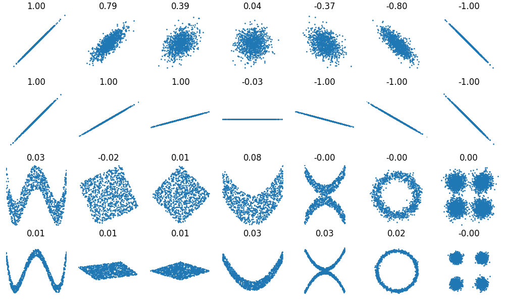
For comparison, we include the results obtained with the standard Pearson correlation, also available in Wikipedia.

fig, axes = plt.subplots(4, 7, **subplot_kwargs)
for (x, y, xlim, ylim), ax in zip(all_datasets(), axes.flat):
    correlation = scipy.stats.pearsonr(x, y).statistic
    plot_data(x, y, ax=ax, xlim=xlim, ylim=ylim)