Performance of the methods

This section shows the relative performance of different algorithms used to compute the functionalities offered in this package.

Distance covariance and distance correlation

We offer currently three different algorithms with different performance characteristics that can be used to compute the estimators of the squared distance covariance, both biased and unbiased.

These algorithms are:

• The original naive algorithm, with order \(O(n^2)\).

• The AVL-inspired fast algorithm described in 1, which improved the performance and attained \(O(n\log n)\) complexity.

• The mergesort algorithm described in 2, which also obtained \(O(n\log n)\) complexity.

The following code shows the differences in performance executing the algorithm 100 times for samples of different sizes. It then plots the resulting graph.

from timeit import repeat

import matplotlib.pyplot as plt
import numpy as np

import dcor

np.random.seed(0)
n_times = 100
n_samples_list = [10, 50, 100, 250, 500, 750, 1000]

avl_times = np.zeros(len(n_samples_list))
avl_uncompiled_times = np.zeros(len(n_samples_list))
mergesort_times = np.zeros(len(n_samples_list))
mergesort_uncompiled_times = np.zeros(len(n_samples_list))
naive_times = np.zeros(len(n_samples_list))

for i, n_samples in enumerate(n_samples_list):
    x = np.random.normal(size=n_samples)
    y = np.random.normal(size=n_samples)

    def avl():
        return dcor.distance_covariance(x, y, method='AVL')

    def avl_uncompiled():
        return dcor.distance_covariance(
            x,
            y,
            method='AVL',
            compile_mode=dcor.CompileMode.NO_COMPILE,
        )

    def mergesort():
        return dcor.distance_covariance(x, y, method='MERGESORT')

    def mergesort_uncompiled():
        return dcor.distance_covariance(
            x,
            y,
            method='MERGESORT',
            compile_mode=dcor.CompileMode.NO_COMPILE,
        )

    def naive():
        return dcor.distance_covariance(x, y, method='NAIVE')

    avl_times[i] = min(
        repeat(avl, repeat=n_times, number=1),
    )
    avl_uncompiled_times[i] = min(
        repeat(avl_uncompiled, repeat=n_times, number=1),
    )
    mergesort_times[i] = min(
        repeat(mergesort, repeat=n_times, number=1),
    )
    mergesort_uncompiled_times[i] = min(
        repeat(mergesort_uncompiled, repeat=n_times, number=1),
    )
    naive_times[i] = min(
        repeat(naive, repeat=n_times, number=1),
    )

plt.title("Distance covariance performance comparison")
plt.xlabel("Number of samples")
plt.ylabel("Time (seconds)")
plt.plot(
    n_samples_list,
    avl_times,
    label="avl",
    linewidth=2,
    marker="o",
)
plt.plot(
    n_samples_list,
    mergesort_times,
    label="mergesort",
    linewidth=2,
    marker="o",
)
plt.plot(
    n_samples_list,
    naive_times,
    label="naive",
    linewidth=2,
    marker="o",
)
plt.legend()
plt.show()

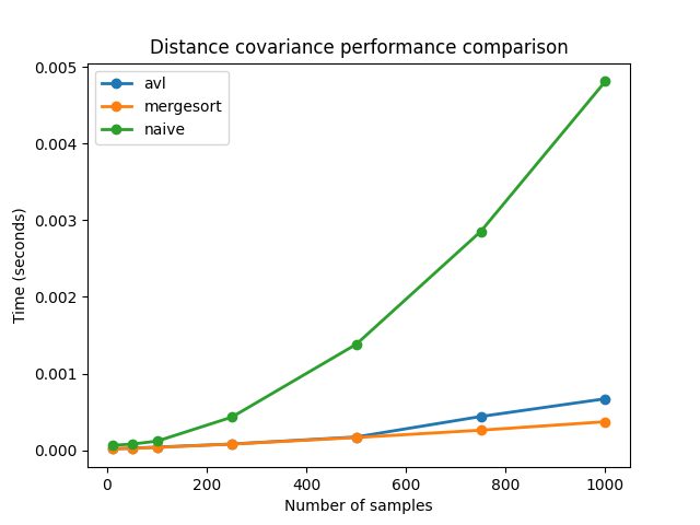
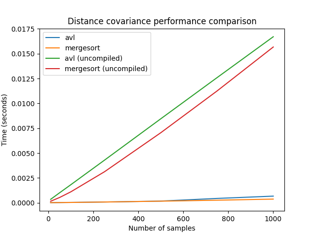
We can see that the performance of the fast methods is much better than the performance of the naive algorithm. We can also check the difference made by the compilation with Numba:

plt.title("Distance covariance performance comparison")
plt.xlabel("Number of samples")
plt.ylabel("Time (seconds)")
plt.plot(n_samples_list, avl_times, label="avl")
plt.plot(n_samples_list, mergesort_times, label="mergesort")
plt.plot(n_samples_list, avl_uncompiled_times, label="avl (uncompiled)")
plt.plot(
    n_samples_list,
    mergesort_uncompiled_times,
    label="mergesort (uncompiled)",
)
plt.legend()
plt.show()

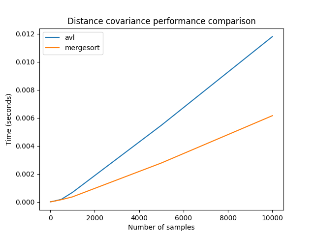
In order to see the differences between the two fast methods, we will again compute them with more samples. The large sample sizes used here could not be used with the naive algorithm, as its used memory also grows quadratically.

n_samples_list = [10, 50, 100, 500, 1000, 5000, 10000]
avl_times = np.zeros(len(n_samples_list))
mergesort_times = np.zeros(len(n_samples_list))

for i, n_samples in enumerate(n_samples_list):
    x = np.random.normal(size=n_samples)
    y = np.random.normal(size=n_samples)

    def avl():
        return dcor.distance_covariance(x, y, method='AVL')

    def mergesort():
        return dcor.distance_covariance(x, y, method='MERGESORT')

    avl_times[i] = min(repeat(avl, repeat=n_times, number=1))
    mergesort_times[i] = min(repeat(mergesort, repeat=n_times, number=1))

plt.title("Distance covariance performance comparison")
plt.xlabel("Number of samples")
plt.ylabel("Time (seconds)")
plt.plot(n_samples_list, avl_times, label="avl")
plt.plot(n_samples_list, mergesort_times, label="mergesort")
plt.legend()
plt.show()

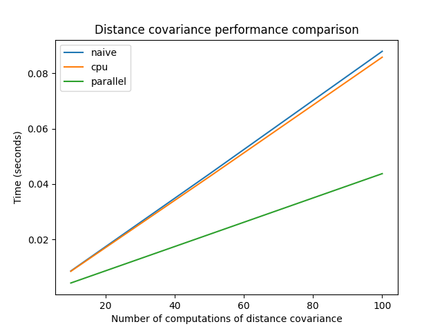
Parallel computation of distance covariance

The following code shows the computation of the distance covariance between several random variables, using the dcor.rowwise() function. If the machine has several CPUs, the time spent using the parallel implementation would be divided by the number of CPUs. If there is only one, there will be no difference.

For now, optimized and parallel implementations are only available for the fast AVL method, which is used by default when the operation is between random variables, and not random vectors.

n_times = 100
n_samples = 1000
n_comps_list = [10, 50, 100]

naive_times = np.zeros(len(n_comps_list))
cpu_times = np.zeros(len(n_comps_list))
parallel_times = np.zeros(len(n_comps_list))

for i, n_comps in enumerate(n_comps_list):
    x = np.random.normal(size=(n_comps, n_samples))
    y = np.random.normal(size=(n_comps, n_samples))

    def naive():
        return dcor.rowwise(
            dcor.distance_covariance_sqr,
            x,
            y,
            rowwise_mode=dcor.RowwiseMode.NAIVE,
        )

    def cpu():
        return dcor.rowwise(
            dcor.distance_covariance_sqr,
            x,
            y,
            compile_mode=dcor.CompileMode.COMPILE_CPU,
        )

    def parallel():
        return dcor.rowwise(
            dcor.distance_covariance_sqr,
            x,
            y,
            compile_mode=dcor.CompileMode.COMPILE_PARALLEL,
        )

    naive_times[i] = min(repeat(naive, repeat=n_times, number=1))
    cpu_times[i] = min(repeat(cpu, repeat=n_times, number=1))
    parallel_times[i] = min(repeat(parallel, repeat=n_times, number=1))

plt.title("Distance covariance performance comparison")
plt.xlabel("Number of computations of distance covariance")
plt.ylabel("Time (seconds)")
plt.plot(n_comps_list, naive_times, label="naive")
plt.plot(n_comps_list, cpu_times, label="cpu")
plt.plot(n_comps_list, parallel_times, label="parallel")
plt.legend()
plt.show()

Bibliography

1

Xiaoming Huo and Gábor J. Székely. Fast computing for distance covariance. Technometrics, 58(4):435–447, 2016. URL: http://dx.doi.org/10.1080/00401706.2015.1054435, arXiv:http://dx.doi.org/10.1080/00401706.2015.1054435, doi:10.1080/00401706.2015.1054435.

2

Arin Chaudhuri and Wenhao Hu. A fast algorithm for computing distance correlation. Computational Statistics & Data Analysis, 135:15–24, July 2019. doi:10.1016/j.csda.2019.01.016.