The distance covariance test of independence

Example that shows the usage of the distance covariance test.

import time

import matplotlib.pyplot as plt
import numpy as np
import pandas as pd

import dcor

# sphinx_gallery_thumbnail_number = 3

Given matching samples of two random vectors with arbitrary dimensions, the distance covariance can be used to construct a permutation test of independence. The null hypothesis \(\mathcal{H}_0\) is that the two random vectors are independent, where the alternative hypothesis \(\mathcal{H}_1\) considers the presence of a (possibly nonlinear) dependence between them.

As an example, we can consider a case with independent observations:

n_samples = 1000
random_state = np.random.default_rng(83110)

x = random_state.uniform(0, 1, size=n_samples)
y = random_state.normal(0, 1, size=n_samples)

plt.scatter(x, y, s=1)
plt.show()

dcor.independence.distance_covariance_test(
    x,
    y,
    num_resamples=200,
    random_state=random_state,
)

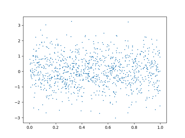
HypothesisTest(pvalue=0.8955223880597015, statistic=0.196086744754483)

Under the null hypothesis, the p-value would have a uniform distribution between 0 and 1. Under the alternative hypothesis, the p-value would tend to 0. Thus, it is common to reject the null hypothesis when the p-value is below a predefined threshold \(\alpha\) (the significance level). There is thus a probability \(\alpha\) of rejecting the null hypothesis even when it is true (Type I error). To ensure that this does not happen often one typically chooses a value for \(\alpha\) of 0.05 or 0.01, to obtain a Type I error less than 5% or 1% of the time, respectively. In this case as the p-value is greater than the threshold we (correctly) don’t reject the null hypothesis, and thus we would consider the random variables independent.

We can now consider the following data:

u = random_state.uniform(-1, 1, size=n_samples)

y = (
    np.cos(u * np.pi)
    + random_state.normal(0, 0.01, size=n_samples)
)
x = (
    np.sin(u * np.pi)
    + random_state.normal(0, 0.01, size=n_samples)
)

plt.scatter(x, y, s=1)
plt.show()

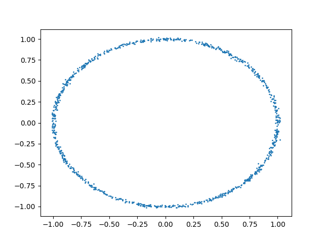
Clearly there is a nonlinear relationship between x and y. We can use the distance covariance test to check that this is the case:

dcor.independence.distance_covariance_test(
    x,
    y,
    num_resamples=200,
    random_state=random_state,
)

HypothesisTest(pvalue=0.004975124378109453, statistic=12.173422287248243)

We can see that the p-value obtained is indeed very small, and thus we can safely reject the null hypothesis, and consider that there is indeed dependence between the random vectors.

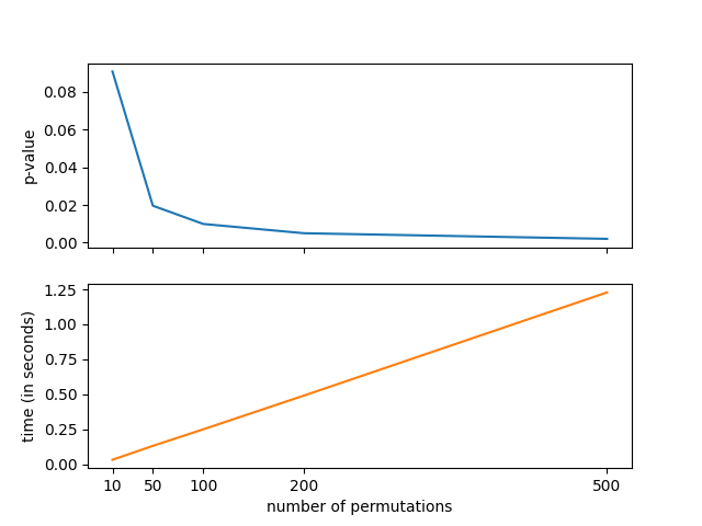
The test illustrated here is a permutation test, which compares the distance covariance of the original dataset with the one obtained after random permutations of one of the input arrays. Thus, increasing the number of permutations makes the p-value more accurate, but increases the computational cost. The following graph illustrates this:

num_resamples_list = [10, 50, 100, 200, 500]

pvalues = []
times = []

for num_resamples in num_resamples_list:

    start_time = time.monotonic()
    test_result = dcor.independence.distance_covariance_test(
        x,
        y,
        num_resamples=num_resamples,
        random_state=random_state,
    )
    end_time = time.monotonic()

    pvalues.append(test_result.pvalue)
    times.append(end_time - start_time)

fig, axes = plt.subplots(2, 1, sharex=True)
axes[0].plot(num_resamples_list, pvalues)
axes[1].plot(num_resamples_list, times, color="C1")
axes[1].set_xticks(num_resamples_list)
axes[1].set_xlabel("number of permutations")
axes[0].set_ylabel("p-value")
axes[1].set_ylabel("time (in seconds)")
plt.show()

In order to check that this test control effectively the Type I error, we can do a simple Monte Carlo test, as explained in the Example 1 of Székely et al.1. What follows is a replication of the results obtained in that example, using a lower number of test repetitions due to time constraints. Users are encouraged to download this example and increase that number to obtain better estimates of the Type I error. In order to replicate the original results, one should set the value of n_tests to 10000.

We generate independent data following a multivariate Gaussian distribution as well as different \(t(\nu)\) distributions. In all cases we consider random vectors with dimension 5. We perform the tests for different number \(n\) of observations, computing the number of permutations used as \(\lfloor 200 + 5000 / n \rfloor\). We fix the significance level to 0.1.

n_tests = 100
dim = 5
n_obs_list = [25, 30, 35, 50, 70, 100]
significance = 0.1


def num_resamples_from_obs(n_obs):
    return 200 + 5000 // n_obs


num_resamples_list = [num_resamples_from_obs(n_obs) for n_obs in n_obs_list]


def multivariate_normal(n_obs):
    return random_state.normal(
        size=(n_obs, dim),
    )


def t_dist_generator(df):
    def t_dist(n_obs):
        return random_state.standard_t(
            df=df,
            size=(n_obs, dim),
        )

    return t_dist


distributions = {
    "Multivariate normal": multivariate_normal,
    "t(1)": t_dist_generator(1),
    "t(2)": t_dist_generator(2),
    "t(3)": t_dist_generator(3),
}
table = pd.DataFrame()
table["n_obs"] = n_obs_list
table["num_resamples"] = num_resamples_list

for dist_name, dist in distributions.items():
    dist_results = []
    for n_obs, num_resamples in zip(n_obs_list, num_resamples_list):
        n_errors = 0
        for _ in range(n_tests):
            x = dist(n_obs)
            y = dist(n_obs)

            test_result = dcor.independence.distance_covariance_test(
                x,
                y,
                num_resamples=num_resamples,
                random_state=random_state,
            )

            if test_result.pvalue < significance:
                n_errors += 1

        error_prob = n_errors / n_tests
        dist_results.append(error_prob)

    table[dist_name] = dist_results

table

	n_obs	num_resamples	Multivariate normal	t(1)	t(2)	t(3)
0	25	400	0.12	0.12	0.05	0.09
1	30	366	0.07	0.05	0.07	0.12
2	35	342	0.09	0.15	0.10	0.08
3	50	300	0.09	0.09	0.09	0.09
4	70	271	0.09	0.12	0.11	0.09
5	100	250	0.10	0.11	0.12	0.09

Bibliography

1

Gábor J. Székely, Maria L. Rizzo, and Nail Kutluzhanovich Bakirov. Measuring and testing dependence by correlation of distances. Ann. Stat., 35(6):2769–2794, December 2007. doi:10.1214/009053607000000505.